A Network, and Where It Starts From

The circuits so far started from nothing and settled. That is fine for a resistor and an inductor, and useless for a network: a real system is already running when you start looking at it, and the transient you care about is the one caused by an event, not by switching the whole grid on.

This tutorial builds a two-bus network, solves its steady state with a powerflow, and starts the dynamic simulation from that solution.

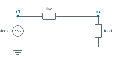
Part one: the powerflow

A powerflow is a different kind of simulation. It has no time step in any meaningful sense; it solves the algebraic steady state, iterating until the bus voltages are consistent with the specified powers.

import dpsimpy
import villas.dataprocessing.readtools as rt

Vnom = 20e3

n1pf = dpsimpy.sp.SimNode("n1", dpsimpy.PhaseType.Single)
n2pf = dpsimpy.sp.SimNode("n2", dpsimpy.PhaseType.Single)

slack = dpsimpy.sp.ph1.NetworkInjection("slack")
slack.set_parameters(voltage_set_point=Vnom)
slack.set_base_voltage(Vnom)
slack.modify_power_flow_bus_type(dpsimpy.PowerflowBusType.VD)

line = dpsimpy.sp.ph1.PiLine("line")
line.set_parameters(R=0.5, L=0.5 / 314, C=50e-6)
line.set_base_voltage(Vnom)

load = dpsimpy.sp.ph1.Load("load")
load.set_parameters(active_power=100e3, reactive_power=50e3, nominal_voltage=Vnom)
load.modify_power_flow_bus_type(dpsimpy.PowerflowBusType.PQ)

slack.connect([n1pf])
line.connect([n1pf, n2pf])
load.connect([n2pf])

system_pf = dpsimpy.SystemTopology(50, [n1pf, n2pf], [slack, line, load])

logger_pf = dpsimpy.Logger("pf")
logger_pf.log_attribute("v1", "v", n1pf)
logger_pf.log_attribute("v2", "v", n2pf)

sim_pf = dpsimpy.Simulation("pf")
sim_pf.set_system(system_pf)
sim_pf.set_domain(dpsimpy.Domain.SP)
sim_pf.set_solver(dpsimpy.Solver.NRP)
sim_pf.set_solver_component_behaviour(dpsimpy.SolverBehaviour.Initialization)
sim_pf.do_init_from_nodes_and_terminals(False)
sim_pf.set_time_step(0.1)
sim_pf.set_final_time(0.1)
sim_pf.add_logger(logger_pf)
sim_pf.run()

Four things here are new and none of them are optional.

The powerflow is built in the static phasor domain, dpsimpy.sp, whatever domain the dynamic run will use. The solver is set to Solver.NRP, the Newton-Raphson powerflow solver, rather than the default nodal solver.

modify_power_flow_bus_type is what makes the problem solvable. Every bus must declare which two of its four quantities are known: VD fixes voltage magnitude and angle, and there must be exactly one such bus, the slack, which absorbs whatever mismatch remains. PQ fixes active and reactive power, which is what a load specifies. Without these the powerflow has no boundary conditions.

set_base_voltage is required on components because the solver works in per unit, and do_init_from_nodes_and_terminals(False) tells the components not to try to initialize themselves from node voltages that do not exist yet, since establishing those voltages is the job this simulation is doing.

Running it gives 20 000 V at the slack and 20 075 V at the load bus. The load bus sitting above nominal is not an error: the line’s shunt capacitance supplies more reactive power at this load than the series impedance drops.

Part two: the dynamic run

The dynamic network is built separately, in the domain the simulation will actually use, and then takes its initial state from the powerflow solution.

n1 = dpsimpy.dp.SimNode("n1", dpsimpy.PhaseType.Single)
n2 = dpsimpy.dp.SimNode("n2", dpsimpy.PhaseType.Single)

slack_d = dpsimpy.dp.ph1.NetworkInjection("slack")
slack_d.set_parameters(V_ref=complex(Vnom, 0))

line_d = dpsimpy.dp.ph1.PiLine("line")
line_d.set_parameters(
    series_resistance=0.5,
    series_inductance=0.5 / 314,
    parallel_capacitance=50e-6,
)

load_d = dpsimpy.dp.ph1.RXLoad("load")
load_d.set_parameters(active_power=100e3, reactive_power=50e3, volt=Vnom)

slack_d.connect([n1])
line_d.connect([n1, n2])
load_d.connect([n2])

system_dp = dpsimpy.SystemTopology(50, [n1, n2], [slack_d, line_d, load_d])
system_dp.init_with_powerflow(systemPF=system_pf, domain=dpsimpy.Domain.DP)

logger = dpsimpy.Logger("dyn")
logger.log_attribute("v2", "v", n2)

sim = dpsimpy.Simulation("dyn")
sim.set_system(system_dp)
sim.set_domain(dpsimpy.Domain.DP)
sim.set_time_step(1e-3)
sim.set_final_time(0.05)
sim.add_logger(logger)
sim.run()

init_with_powerflow matches the two networks by node name and copies the solved voltages across, which is why the node names must agree between the two topologies. It is the only line connecting the two halves.

The result is the point of the whole exercise. The dynamic run starts at 20 074.8 V and ends at 20 074.9 V: it begins in steady state rather than settling into one. Without the powerflow it would start from zero and spend the first several cycles charging the line, and any event applied during that period would be mixed in with a startup transient that has nothing to do with the system.

Parameter names differ between domains

The same component takes different keyword names in different domains. The static phasor line takes R, L and C; the dynamic phasor line takes series_resistance, series_inductance and parallel_capacitance. The load is Load with nominal_voltage in the powerflow and RXLoad with volt in the dynamic run.

The script

The complete script for this page is 03_two_bus_network.py under examples/Python/Tutorials. The numbers quoted above are the numbers it prints, so if the two ever disagree the page is the one that is wrong.

Next

The network now starts where it should, so an event applied to it produces a clean response. Next is applying one: a fault, using a switch.

The powerflow method is described under powerflow, and the loads and lines used here under loads and branches.