Your First Simulation

This page goes from nothing to a plotted result. It assumes DPsim is installed and importable; if it is not, start with install or build.

The circuit is deliberately trivial, a voltage source feeding a resistor, so that nothing in it distracts from the shape of the script. Every real simulation has the same five parts in the same order.

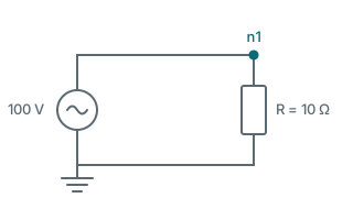
The whole script

import dpsimpy
import villas.dataprocessing.readtools as rt
from villas.dataprocessing.timeseries import TimeSeries as ts

name = "first_simulation"

# 1. Nodes
gnd = dpsimpy.dp.SimNode.gnd
n1 = dpsimpy.dp.SimNode("n1")

# 2. Components
src = dpsimpy.dp.ph1.VoltageSource("src")
src.V_ref = complex(100, 0)

load = dpsimpy.dp.ph1.Resistor("load")
load.R = 10.0

# 3. Connections
src.connect([gnd, n1])
load.connect([n1, gnd])

# 4. Topology
system = dpsimpy.SystemTopology(50, [gnd, n1], [src, load])

# 5. Logging, then run
logger = dpsimpy.Logger(name)
logger.log_attribute("n1.v", "v", n1)
logger.log_attribute("load.i_intf", "i_intf", load)

sim = dpsimpy.Simulation(name)
sim.set_domain(dpsimpy.Domain.DP)
sim.set_system(system)
sim.set_time_step(1e-3)
sim.set_final_time(0.1)
sim.add_logger(logger)
sim.run()

Running it prints solver progress and writes logs/first_simulation.csv.

What each part is doing

Nodes come first because components connect to them, not to each other. SimNode.gnd is the reference node and is shared; every network needs it. Nodes are chosen from a domain namespace, dpsimpy.dp here, and a node from one domain cannot be connected to a component from another.

Components are created, then configured through their attributes. src.V_ref = complex(100, 0) sets the source reference as a complex phasor, because this is the dynamic phasor domain and a voltage is an envelope rather than an instantaneous value. In EMT the same field would carry a different meaning; see dynamic phasors.

Logging is opt-in, and takes three steps in order. Nothing is recorded unless a logger asks for it.

logger = dpsimpy.Logger(name)                          # 1. create it; the name becomes the file name
logger.log_attribute("n1.v", "v", n1)                  # 2. register each attribute you want
logger.log_attribute("load.i_intf", "i_intf", load)
sim.add_logger(logger)                                 # 3. attach it to the simulation, before run()

log_attribute takes the column name you want, the name of the attribute on the object, and the object itself. "v" on a node is its voltage; "i_intf" on a component is the current through it. The first argument is yours to choose and is the key you will use when reading the file back; the second must be an attribute the object actually publishes, and print_attribute_list() on the object shows what that is.

The order is what makes it work. A logger registers attributes before it is attached, and it must be attached before run(), because the column header is written from whatever is registered when the first row is written. A logger created but never passed to add_logger produces no file at all, which is the usual reason for a run that appears to have logged nothing.

Reading the results

results = rt.read_timeseries_dpsim("logs/" + name + ".csv")

print(sorted(results.keys()))
# ['load.i_intf', 'n1.v']

v = results["n1.v"]
print(v.time[1], abs(v.values[1]))
# 0.001 100.0

The keys are the column names given to log_attribute. Each value is a time series with time and values arrays; in a dynamic phasor simulation the values are complex, and abs() gives the envelope magnitude.

Note that the first sample is zero. The log is written before the first solve, so row zero is the state the simulation started from rather than a result. From t = 0.001 onwards this circuit sits at exactly 100 V and 10 A, which is what a 100 V source across 10 Ω should give.

Plotting

import villas.dataprocessing.plottools as pt

pt.plot_timeseries(1, results["n1.v"].abs())
pt.plot_timeseries(2, results["load.i_intf"].abs())

The first argument is a figure number, so repeated calls with the same number overlay curves on one axis. .abs() is needed for complex results; plotting a complex series directly is not meaningful.

Recovering the waveform from a dynamic phasor result

A dynamic phasor result is an envelope, not a waveform. To compare it against an instantaneous result, shift it back onto the carrier:

emt = ts.frequency_shift_list(results, 50)
print(sorted(emt.keys()))
# ['load.i_intf_shift', 'n1.v_shift']

The script

The complete script for this page is 01_first_simulation.py under examples/Python/Tutorials. The numbers quoted above are the numbers it prints, so if the two ever disagree the page is the one that is wrong.

Next

This circuit has no dynamics at all: it is a source and a resistor, so it reaches its final value in one step and stays there. The next step is to add an element that stores energy, which is where the choice of time step starts to matter and where a result becomes worth plotting.

The examples work through larger networks, and the models used here are derived under sources and RLC elements.