The Same Circuit in Two Domains
Every result so far has been an envelope, and the pages have said that an envelope is not a waveform without showing what the difference costs. This tutorial runs the same circuit both ways and puts the two on one axis.
The circuit is the RL branch from adding dynamics, unchanged.
Building the same circuit twice
Only the namespaces differ. dpsimpy.emt.ph1 instead of dpsimpy.dp.ph1, and Domain.EMT instead
of Domain.DP:
def build(domain, ns, ph1, name, dt):
    gnd = ns.SimNode.gnd
    n1 = ns.SimNode("n1")
    n2 = ns.SimNode("n2")

    src = ph1.VoltageSource("src")
    src.set_parameters(
        V_ref=complex(100, 0),
        f_src=(50.0 if domain == dpsimpy.Domain.EMT else 0.0),
    )

    r = ph1.Resistor("r"); r.set_parameters(R=10.0)
    l = ph1.Inductor("l"); l.set_parameters(L=0.05)

    src.connect([gnd, n1]); r.connect([n1, n2]); l.connect([n2, gnd])

    system = dpsimpy.SystemTopology(50, [gnd, n1, n2], [src, r, l])
    logger = dpsimpy.Logger(name)
    logger.log_attribute("i_l", "i_intf", l)

    sim = dpsimpy.Simulation(name)
    sim.set_domain(domain); sim.set_system(system)
    sim.set_time_step(dt); sim.set_final_time(0.06)
    sim.add_logger(logger)
    sim.run()
    return rt.read_timeseries_dpsim("logs/%s.csv" % name)

emt = build(dpsimpy.Domain.EMT, dpsimpy.emt, dpsimpy.emt.ph1, "cmp_emt", 5e-5)["i_l"]
dp = build(dpsimpy.Domain.DP, dpsimpy.dp, dpsimpy.dp.ph1, "cmp_dp", 1e-3)
dp_shift = ts.frequency_shift_list(dp, 50)["i_l_shift"]
The one parameter that means different things
f_src is not the same quantity in the two domains, and this is the single easiest way to get a
wrong answer here.
Watch out: f_src means different things per domain
In EMT it is the absolute frequency of the source, so 50 Hz means 50 Hz. In DP and SP it is an offset from the carrier, so passing 50 there gives a source at 100 Hz. Leave it at zero, or omit it, when you want a source at the system frequency in an envelope domain.
Getting this wrong is not obvious from the output: the simulation runs, and the current is simply smaller than it should be because the inductive reactance has doubled. In this circuit the wrong setting gives 3.02 A instead of 5.37 A, which looks like a plausible number rather than an error.
The comparison
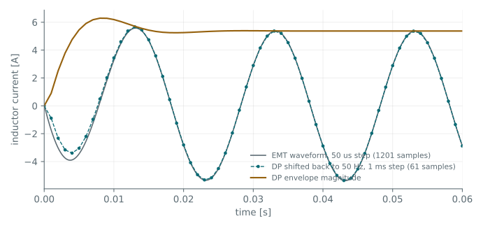
The dashed line is the dynamic phasor result shifted back onto the 50 Hz carrier. It lies on the EMT waveform. The third curve is the envelope magnitude itself, which is what the DP simulation actually computed: the smooth rise to 5.37 A that the oscillation is riding on.
| Quantity | EMT | DP shifted back |
|---|---|---|
| Time step | 50 µs | 1 ms |
| Samples over 60 ms | 1201 | 61 |
| Peak current, steady state | 5.3703 A | 5.3603 A |
| Current at t = 60 ms | −2.8839 A | −2.8840 A |
Twenty times fewer steps, and the same answer to four significant figures.
Why this works, and when it does not
The saving is not because the envelope model is coarser. For a single carrier the transform is exact. The 50 Hz oscillation has been moved out of the integrated quantity and into a coefficient handled analytically, so the step size is set by how fast the envelope changes rather than by the carrier. Here the envelope settles with a 5 ms time constant, and 1 ms resolves it comfortably.
What an envelope domain cannot represent is content outside the band it retains around the carrier. A harmonic, a fast switching transient, or a wideband disturbance is simply absent. That is the trade, and it is the reason both domains exist rather than one being better.
The transform itself is derived under dynamic phasors.
Reading it back
frequency_shift_list appends _shift to every key, so the shifted series is i_l_shift and not
i_l. Asking for the original name after shifting raises a KeyError that reads like a missing
signal.
The script
The complete script for this page is 05_comparing_domains.py under examples/Python/Tutorials. The numbers quoted above are the numbers it prints, so if the two ever disagree the page is the one that is wrong.
Next
The circuits so far have been passive. Next is a synchronous machine, where the model order becomes a choice and initialization from a powerflow stops being optional.